Overview
During my
Continuous
Futures project I was already impressed by the capabilities of
Plotly with regards to all the nice interactivity it brings to data
visualisation. In combination with Cufflinks it turned out to be an
even more powerful tool for handling financial data. A little
drawback, at least for somebody who is a trader in the first place,
was the tricky embedding of those Plotly objects into web based environments. Later, when I was designing on more
complex visualisations, with different tables, graphs etc. that are
all linked together and therefore causing a lot of dependencies, I was
obviously missing a powerful tool to achieve that. The solution,
Dash, was such a good fit that I decided to write this article as a
little introduction to it.
What makes Dash so powerful in financial applications?
Basically you can create web apps that completely run in the browser without any knowledge of HTML or JavaScript. The range of capabilities is quite impressive as it goes from simply hosting a Plotly graph up to building a front-end for an algorithmic trading system with dozens of dependencies, different tabs, real-time charts, PnL monitoring etc. It can also make those tons of circulating financial market research in PDF format much more interactive. Just imagine you could tweak those reports a little: like substitute one time-series for another, zoom-in to a particular area of a chart or simply hover over it to get the precise data reading. You could even make whole text phrases dependent on what assumptions the reader is making (e. g. growth rates, inflation or FX rates in a macroeconomic model).
But let’s see all this in a little example…
…based on my previous work on Continuous Futures. This
series was about the implication of price gaps between
subsequent futures contracts and how to take care of them when it
comes to trading and research. Now we let the user explore the dataset
on his own by letting him choose a futures position and then giving
him immediate feedback with all the analytics from the original
research article.
For our Dash app, we therefore implement functionality along the following
lines:
-
User inputs
-
Futures contract type
-
Buy or sell Futures
-
Amount of contracts
-
Investment period
-
-
Output of the following figures with and without roll adjustment
-
PnL differences
-
Closing price chart over investment period
-
Candlestick charts with technical trading indicators
-
Trading signal differences
-
But before we dive into the technical details of how to deploy such an app, let’s take a look at it:
The basic structure of a Dash app
Typically the first thing you would take care of in deploying a Dash
app is getting a broad idea of how the layout would look like. For me
the most convenient way to deal with that is using an external style
sheet that breaks the appearance on the screen down into rows and
columns. Styling within that style sheet is then feasible with a Dash
component called HTML Components. The content or the data you want
to visualize will also be embedded along the coordinates of the style
sheet, but sits in another part of the Dash library: the Dash Core
Components. Those are for example drop-down menus, sliders, text
fields, graphs, tables and many more. Now the part that links
everything together and brings all the interactivity to it are
Callbacks. Callbacks have (multiple) inputs, an automatically called
function for the processing, and finally an output that updates the
dashboard. This typically involves interaction with a Plotly object
like a graph or a table. The nice thing about that is, if you are
familiar with Plotly, the new dimension with Dash is just structuring
how Plotly objects behave and how they interact in the context of the
dashboard. The object itself is identical to what you already have
done with Plotly. Now we look at the outlined building blocks of the
app in more detail.
Library imports
Libraries to run Dash:
import dash
from dash.dependencies import Input, Output, State, Event
import dash_core_components as dcc
import dash_html_components as html
Additional libraries for our app:
import plotly
import cufflinks as cf
import flask
import numpy as np
import pandas as pd
import pickle
from datetime import datetime as dt
from pandas.tseries.offsets import DateOffset
Styling the app
Embedding the external style sheet:
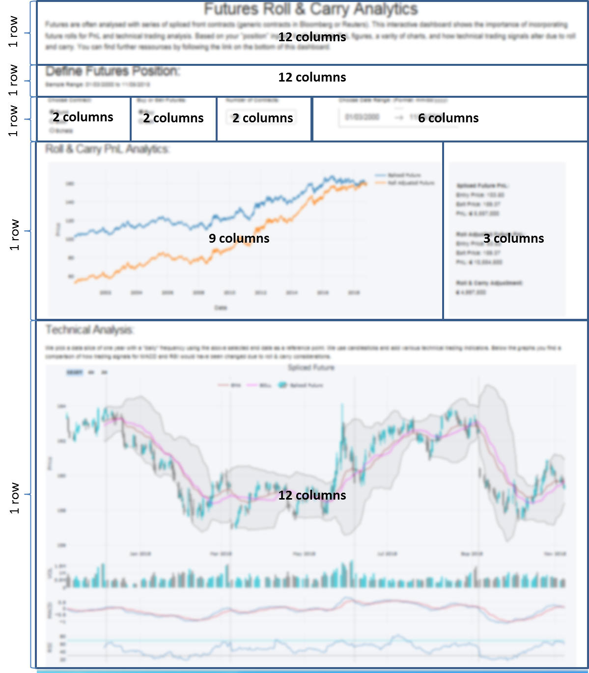
app.css.append_css({'external_url': 'https://cdn.rawgit.com/plotly/dash-app-stylesheets/2d266c578d2a6e8850ebce48fdb52759b2aef506/stylesheet-oil-and-gas.css'})The above CSS style sheet gives our app structure that is best thought of as dividing everthing into rows and columns. While rows are simply appended, columns have to add up to 12 (e.g. 3 + 9, 5 + 5 + 2, …). On each intersection of row y and column x you typically find an object like a graph. The illustrations below will shed some light on how CSS styling was utilized in our app.
We open the styling as follows (we make use of "Dash HTML Components" here):
app.layout = html.Div([
    # Title + Description
    html.Div(
        [
            html.H1(
                'Futures Carry Analytics',
                style={'font-family': 'Helvetica',
                       "margin-top": "25",
                       "margin-bottom": "0"},
            ),
            html.P(
                'Futures are often analysed with series of spliced front contracts. This interactive dashboard shows the importance of incorporating Future rolls for PnL and technical trading analytics.',
                style={'font-family': 'Helvetica',
                       "font-size": "120%",
                       "width": "100%"},
            ),
        ],
        className='row'
    ),
...
The above code piece represents the first row of our app. All other
rows are simply appended to the one that was defined before. We now
skip row number two and directly go to the third one because that is a
user input utilizing one of the Dash Core Components, a radio item
in this case.
User chooses contract:
...
html.Div(
                [
                    html.P('Choose Contract:'),
                    dcc.RadioItems(
                        options=[
                            {'label': 'Bund', 'value': 'FGBL'},
                            {'label': 'Bobl', 'value': 'FGBM'},
                            {'label': 'Schatz', 'value': 'FGBS'}
                            ],
                        value='FGBL',
                        id = 'radioitem_future'
                        )],
                        className = 'two columns',
                        style = {'margin-top': '10'}
                        )
...
The code above represents the first two columns in row number three. The graph responding to the inputs in row three is located one row below.
Graph updating according to the user inputs:
...
html.Div([
                    dcc.Graph(
                    id='Futures Graph',
                    )
                ]
...
All other objects are inserted into the style sheet in a similar fashion.
Adding interactivity with callbacks
Now we add a layer to our code that connects user inputs with applying
the needed updates on our output objects. This is done with a callback
decorator that automatically calls a function whenever the state of a
pre-defined input changes. The called function itself then updates the
property of the output object. The callback below updates two
time-series in the graph we have seen above that was dependent on the selection of an underlying
future along with a selected start and end date.
@app.callback(
    Output('Futures Graph', 'figure'),
    [Input('radioitem_future', 'value'),
     Input('date_range_future', 'start_date'),
     Input('date_range_future', 'end_date')])
def update_graph(value, start_date, end_date):
    figure={
        'data': [
            {'x': data_dict[value]['Front'][start_date:end_date].index,
                'y': data_dict[value]['Front'][start_date:end_date]['CLOSE'],
                'type': 'line', 'name': 'Spliced Future'},
            {'x': data_dict['%s_pan' % value][start_date:end_date].index,
                'y': data_dict['%s_pan' % value][start_date:end_date]['CLOSE'],
                'type': 'line', 'name': 'Roll Adjusted Future'}
            ],
            'layout': {
                'title': 'Spliced vs. Roll Adjusted Futures',
                'xaxis': {'title': 'Date'},
                'yaxis': {'title': 'Futures Price'}
                }
            }
    return figure
Now we have already everything together to make our app work.
Advanced Dash features
Although the above steps are fully sufficient to get our app going, we
will make use of some more advanced techniques to make it
computationally more efficient. For that purpose we will focus on
Buttons which enable controlling the launch of "expensive"
computations via a dependency called State. Another efficiency gain
is sharing time-consuming calculations between callbacks with a
Hidden Div.
Buttons
Regular Dash inputs recognise a (user) change of the input object
immediately and then kick-off the associated callback(s). In many
cases the user specifies multiple inputs and a computation is only
needed when all inputs are completed. The dependency State makes it
now possible to fire callbacks dependent on pressing a Button. In
our app we use this concept to let the user specify a futures
position completely and only then submit it for the needed
calculations. Below you can see how the button was added to the
inputs area of the dashboard:
...
html.Button('Submit', id='button', style={'margin-top': '30'}),
],
    className = 'two columns',
    style = {'margin-top': '10'}
    ),
...
To make a callback reactive to pushing the button, we have to change it a bit:
...
@app.callback(
    Output('Futures Graph', 'figure'),
    [Input('button', 'n_clicks')],
    state=[State('radioitem_future', 'value'),
     State('date_range_future', 'start_date'),
     State('date_range_future', 'end_date')])
...
Maybe you have already noticed that this is the new version of the
graph callback from above. We have simply changed Input to the
button and the items that have been inputs before, are now type
State. That is just holding back the execution of the function
belonging to the callback until the button was hit.
Sharing Data between Callbacks
At a first glance it might look appealing to use global variables for
shared data. As Dash is used in multi-user environments and is also
able to run with multiple Python workers, global variables can be
critical and should never be modified by callbacks. A better way
is using a Hidden Div that uses a callback to provide calculation
tasks that other callbacks can also use without the need for them to
replicate those calculations themselves. The information shared is of type JSON. Here is the Hidden Div as
specified in the layout section:
...
html.Div(id='pre-processing', style={'display': 'none'}),
...
Now we make our "complex" calculations in a single callback:
...
@app.callback(
Output('pre-processing', 'children'),
[Input('button', 'n_clicks')],
state=[
 State('radioitem_future', 'value'),
 State('date_range_future', 'end_date')])
def preparation(n_clicks, future, end_date):
  '''Now the complex calculation....'''
    return json.dumps(tech_charts, cls=plotly.utils.PlotlyJSONEncoder)
...
Other callbacks now make use of it as simple as that:
...
@app.callback(
    Output('Spliced Technical Graph', 'figure'),
    [Input('pre-processing', 'children')])
def update_graph(json_file):
    figure = json.loads(json_file)
    figure = figure['spliced']
    return figure
...
Deploying Dash Apps
By default your Dash app runs on Localhost. This means it is only
available on your own machine. Typically you will use this mode in
development and for testing. As soon as you want to make your app
public, it has to sit on a server that is open for outside access. To
make this happen, Dash uses Flask which in turn is supported by a wide
range of cloud server providers. On the Dash website you can find a
nice tutorial on how to
"deploy" with Heroku.
I hope you have enjoyed reading this little tutorial and you are more than welcome to get in touch via the comment section or a personal message.